SPECFEM has been a cornerstone of computational seismology for over two decades. The Fortran-based software suite is used for seismic wave propagation simulations and adjoint tomography, accumulating thousands of citations per year across a broad user base. But the original codebase grew across three separate repositories (2D, 3D, and 3D Globe) with substantial redundancy and architecture-specific GPU kernels, meaning new features rarely made it to all variants.
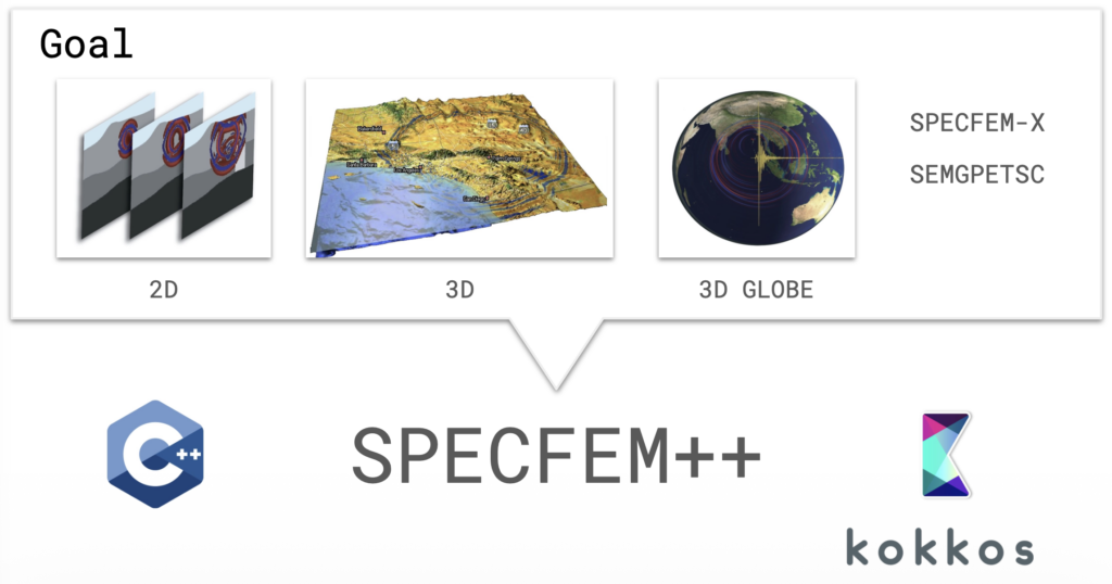
SPECFEM++ is the solution: a ground-up rewrite in C++ using Kokkos for performance portability across CPUs, NVIDIA GPUs (CUDA), and AMD GPUs (HIP) — all from a single codebase.
Expanded Physics
One of the primary goals of SPECFEM++ is to make adding new physics straightforward. The solver now supports elastic P-SV and SH waves, anisotropic media, poroelastic domains, and Cosserat media (which adds rotational degrees of freedom alongside displacement). Most significantly, 3D elastic isotropic simulation is now fully supported, with end-to-end integration tests confirming sample-by-sample agreement with SPECFEM3D Cartesian.
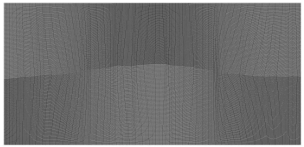
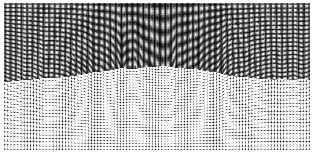
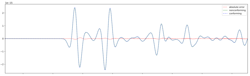
For problems with large contrasts in physical properties, non-conforming mesh support via a Discontinuous Galerkin approach allows different element sizes on either side of an interface. This enables the code to choose larger timesteps and drastically improve performance.
Conforming mesh with bathymetry.Non-Conforming Mesh.Associated Non-conforming simulation. The conforming simulation is part of Pipatprathanporn et al., 2024 (DOI). Credit: Kentaro G. Hanson (G3, PACM).Seismograms for conforming and nonconforming DG simulation as well as associated error. Credit: Kentaro G. Hanson (G3, PACM).
Performance on Par with — and Beyond — SPECFEM2D
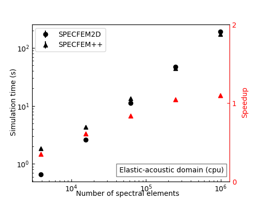
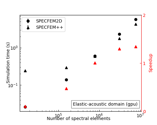
After memory layout optimizations, SPECFEM++ now matches SPECFEM2D on CPU for elastic and acoustic problems. On GPU, it pulls ahead: for large elastic-acoustic domains (10M+ spectral elements), SPECFEM++ achieves up to 2× speedup over SPECFEM2D.
Performance comparison between SPECFEM2D Fortran and SPECFEM++ on CPU.Performance comparison between SPECFEM2D Fortran and SPECFEM++ on GPU.
Real-World Benchmarks: Marmousi and Cosserat
Two showcases stand out. The Marmousi model cookbook runs wave propagation on a high-resolution CUBIT mesh derived from a classic seismic benchmark, and is a great stress test of the GPU backend. The Cosserat media simulation illustrates the rotational wavefield alongside displacement — something not possible in the original SPECFEM.
Wave propagation due to an isotropic, explosive source in the complex Marmousi model. Water (acoustic) layer on top and a complex, solid layer below with Stacey Boundary conditions.Wave propagation in a homogeneous Cosserat medium with Stacey boundary conditions on all sides. Left: Magnitude of the displacement component. Right: Rotational (spin) component. Credit: Max Chien (Junior, PACM).
Tooling and Documentation
Nightly benchmarks run automatically via Jenkins on Intel Gold CPUs and
NVIDIA H100 GPUs, with results on a live review
dashboard.
The API documentation now includes the actual implemented equations, and
cookbooks cover everything from basic homogeneous media to non-conforming
fluid-solid interfaces.
What’s Next
Active development is focused on MPI support, attenuation, and acoustic-elastic
coupling — the remaining pieces needed for large-scale parallel 3D production
runs.
SPECFEM++ is a community project with monthly developer meetings (first Wednesday of each month, 12:00 PM Eastern sign up here). Documentation is at specfem2d-kokkos.readthedocs.io and the code is on GitHub.
Acknowledgements: The initial draft for this post was generated by Anthropic’s Claude Sonnet 4.6 using presentation slides and github release notes.
ASPIRE is an open-source Python package for 3D molecular structure determination using cryo-EM with many submodules solving complex equations that could be accelerated on GPUs. ASPIRE developers have participated in GPU hackathons for the last 4 years, but new group members Josh and Chris attended for the first time this year. The problem selected by Josh and Chris was spectral decomposition using the power method for determining leading eigenvalue/eigenvector – a limiting step in ASPIRE’s computation pipeline. The problem was ideal in scope, tested and provided a range of problem sizes for scaling experiments onto a GPU. The team primarily worked by pair programming, frequently meeting together to share paired results and determine next steps.
Resolving Python Anti-Patterns
The initial implementation had a few “fast python anti-patterns”. On the first day, we replaced for-loops and Python list comprehensions with NumPy operations for large speedups, even before moving to a GPU. We used Python’s standard library profiler, cProfile to get an idea of the functions slowing down the code. We visualized the profiler output using SnakeViz.
Figure 1: Python cProfile of the original implementation visualized with SnakeViz.
Moving to CuPy
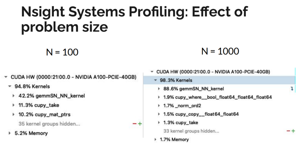
We initially used drop-in replacements of NumPy calls with CuPy. This actually worsened performance compared to a single CPU core, likely because optimizations for CPU do not necessarily translate to GPU speedups. We used NVIDIA’s Nsight Systems to generate a profile of the kernel launches being generated by CuPy and understand the memory transfers from host to device. We noticed that CuPy was generating hundreds of launches of a kernel called “gemmSN_NN_kernel”. Although each call performed a small operation, the launch time overhead was as costly as the operation itself. In aggregate, these launches added up significantly, and–worse–this issue would scale with problem size. Further analysis showed that the large number of kernel launches generated by CuPy was due primarily to two operations. First, a 4D matrix multiply was decomposed into a series of 3D multiplications, where the last dimensions were small. Flattening the matrix into 3D greatly reduced the number of kernel launches and increased the size of each operation. Second, a matrix conjugation was expressed as a direct translation of the underlying mathematical theory as two matrix multiply operations. Careful inspection of the final result revealed the costly multiplications could be replaced with a single, element-wise multiplication, further reducing the number of kernel launches performed by CuPy.
Figure 2: Nvidia Nsight Systems breakdown of naive drop-in CuPy replacement showing costly matrix multiply kernel launches.
Randomizing Batch Operation
As part of refactoring, we had modified the index generator to produce subproblems in batches, instead of individually. The batch size is derived from the problem size and the indices were generated in sorted order. This caused a memory bottleneck during a final sum-reduce operation that was expressed as a weighted histogram function. The sorted indices were causing collisions into bins, leading to inefficient memory access due to the required atomicAdd when accumulating into one bin. We addressed this slowdown by randomizing the indices that are batched together to decrease the frequency of stalls during the reduce operation. We also identified that we could cache the indices for each iteration, further accelerating the code.
Figure 3: Histogram of hit counts for each iteration in the loop (a) indices generated in sorted order shows each loop updating a small number of positions causing collisions (b) randomizing the indices that are batched together decreases the frequency of stalls during the reduce operation.
Host Memory Bug
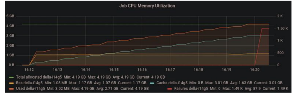
As we ramped up the problem size, we noticed that we were running out of memory on the host machine after a few iterations. Since the code was performing all operations in-place, the accumulating host memory was initially mysterious.
Figure 4: Increasing memory utilization in the host machine suggesting a memory leak.
We tracked down the issue to a temporary variable overriding a variable that was used outside the loop scope in the outer iteration of the power method. In the code below, “vec” is initialized before the loop. On each iteration, “vec” is replaced with “vec_new” and the old value of “vec” can be safely discarded. However, since “vec” is used after the loop, CuPy retained a copy of “vec” on the host memory, causing copies of “vec” to accumulate.
    # Power method iterations
    for itr in range(max_iters):
        vec_new = signs_times_v(vijs, vec, conjugate, edge_signs)
        vec_new /= norm(vec_new)
        residual = norm(vec_new - vec)
        vec = vec_new
        if residual < epsilon:
            print(f'Converged after {itr} iterations of the power method.')
            break
    else:
        print('max iterations')

    # We need only the signs of the eigenvector
    J_sync = np.sign(vec)
The simple solution was to initialize vec_new before the loop and use its value after the loop exits so that CuPy knows “vec” can be safely garbage collected in each iteration.
# initialize vec_new to prevent blocking garbage collection of vecvec_new = vec
# Power method iterations
for itr in range(max_iters):
triplets_iter = all_triplets_batch(triplets, batch_size)
vec_new = signs_times_v(vijs, vec, conjugate, edge_signs, triplets_iter)
vec_new /= norm(vec_new)
residual = norm(vec_new - vec)
vec = vec_new
if residual < epsilon:
print(f'Converged after {itr} iterations of the power method.')
break
else:
print('max iterations')
# We need only the signs of the eigenvector
J_sync = np.sign(vec_new)
Final Speedup
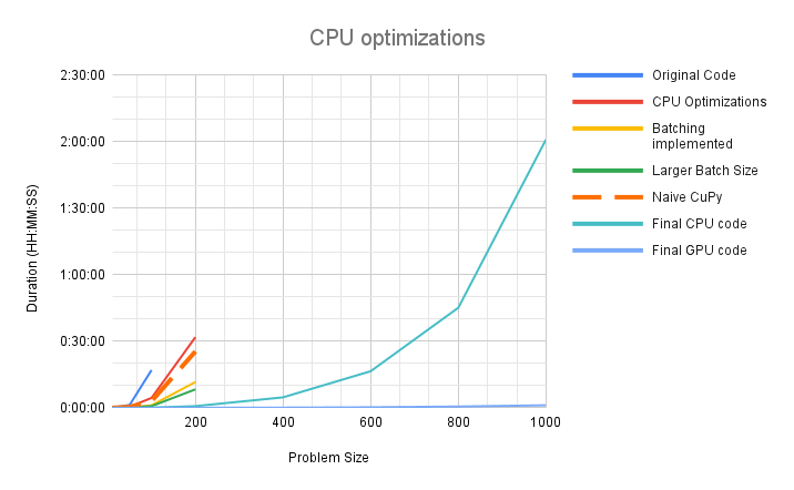
We achieved significant speedup on both CPU and the GPU. In our initial implementation the code would timeout after 4 hours, processing a problem size of N=400. After all optimizations, we are processing a realistic problem size of N=1000 in 2 hours on CPU and just over 1 minute on the GPU. The problem sizes that needed to be partitioned before can now be executed directly and the implementation is expected to scale to larger problem sizes as well.
Figure 5: Performance scaling chart showing improvement in both the serial and GPU versions. The serial version is estimated to have 30x speedup over the original version and the GPU accelerated version has a further speedup of 120x over the serial version.
Takeaways
There were some key points that we feel were essential to achieving these improvements within the constraints of a 4-day hackathon.
Preparation
It was crucial that the target algorithm could be run and tested in isolation, away from the rest of the codebase. Our algorithm is an intermediate step within a large computational pipeline. It would be difficult to quickly test modifications and pinpoint optimizations in the full problem context, so the algorithm was broken out of the main code and put into a standalone script. We also wrote a script to generate sample inputs of any problem size, which could be created and saved to disk outside of the code to be optimized. The key here is to identify what external information your code needs to run in a realistic setting, and try to eliminate everything else. In addition, as a sanity check, we saved *outputs* of the original code for comparison, in case our modifications unintentionally broke the code.
Don’t prematurely optimize
A lot of code is not initially written to be maximally efficient; there is often a trade-off between readability and efficiency. Correctness and communicating an algorithm are vital for code when it is first written. Look for common improvements to be made before attempting to profile the code on the GPU. For example, using cProfile we found bloated Python code that was easy to streamline without resorting to fancy solutions. Removing unnecessary list comprehensions and directly calculating indices instead of searching for them led to large speedups without sacrificing readability. Next, we optimized the code to run just on the CPU by translating verbose, multi-step calculations with more terse, single calls to NumPy routines. As a bonus, code that primarily uses NumPy is easy to translate into CuPy. Finally, we moved on to the GPU, confident that we were entering this stage of the hackathon with robust, vetted code. There are options for when code starts to become cryptic. Commenting code that has become too obtuse with the original, verbose version is an easy way to retain documentation. Moving the old version into a unit test is a more active way to ensure new versions continue to match legacy code while providing some documentation.
Working as a Group
Having two pair programming teams tackling a complicated piece of numerical code requires coordination. In addition to isolating all the code and data we needed to experiment, we put all of this into a git repository. With each pair working on an individual feature branch, along with asynchronously communicating via Slack, collisions and confusion were avoided. As mentioned above, optimization can make code more difficult to read, so verbal briefings of how and why changes were made kept everyone on the same page.
APPLE-Picker is a submodule of ASPIRE Python package in development for reconstructing a 3D CryoEM map of biomolecule from corresponding 2D particle images, developed by the researchers in Professor Amit Singer’s group. It is an automatic tool to select millions of particles from thousands of micrographs, a critical step in the pipeline of CryoEM image reconstruction. It used to be performed manually but can be very tedious and difficult especially for small particles with low contrast (low signal-noise ratio). The CPU version takes ~80 seconds on average to finish processing one micrograph. To achieve the goal of finishing thousands of micrographs in a few minutes, we need an alternative method, such as GPU accelerating.
2019 Princeton GPU Hackathon
Princeton university held its first GPU hackathon on campus this summer from June 24 to 28, organized and hosted by the Princeton Institute for Computational Science and Engineering (PICSciE), and co-sponsored by NVIDIA and the Oak Ridge Leadership Computing Facility (OLCF). The main goal of this Hackathon was to port research codes to GPUs or optimize them with the help of experts from industry, academia and national labs, as emphasized by Ian Cosden, one of lead organizers and manager of Princeton’s Research Software Engineering Group. This blog reports our attempts and the story behind accelerating APPLE-Picker using GPU and parallel computing in Python.